Guide to Gradient Descent in 3 Steps and 12 Drawings
Everyone knows about gradient descent. But… Do you really know how it works? Have you already implemented the algorithm by yourself?
Using modules and all, it’s cool.
But understanding what’s behind the python functions, it’s way better!
In this article, I’ll guide you through gradient descent in 3 steps:
- Gradient descent, what is it exactly?
- How does it work?
- What are the common pitfalls?
The only prerequisite to this article is to know what a derivative is.
What is Gradient Descent?
It is an algorithm used to find the minimum of a function.
That’s called an optimization problem and this one is huge in mathematics.
It’s also the case in data science, especially when we’re trying to compute the estimator of maximum likelihood.
The kind of thing we’re doing every day.
Oh and.. of course, finding a minimum, or a maximum, it’s the same thing. You only need to change the sign.
.
Remember high school?
You learned a way to find the minimum of a function:
- Compute the first-order derivative.
- Solve the equation derivative = 0 to find the inflection points.
- Compute the second-order derivative in these points. When it’s positive, it’s a minimum. If it’s negative, it’s a maximum.
Ok, cool.
This technique works well.
EXCEPT…
…when the functions are so complex that it’s impossible to solve!
Typically when you’re doing machine learning or deep learning.
In these cases, we do gradient descent. That’s an approach:
- algorithmic
- iterative
- that works rather well in most cases
I’m adding this last point because sometimes it doesn’t work. Fortunately, there are extensions to solve these issues.
We won’t discuss them too much in this article, but we’ll see the most common problems you will probably encounter.
How does it work?
Let’s start with an intuitive explanation. Then we’ll do the math.
Imagine you are a skier on a mountain.
And you want to find the lowest point around you, i.e. finding the place with minimal altitude.
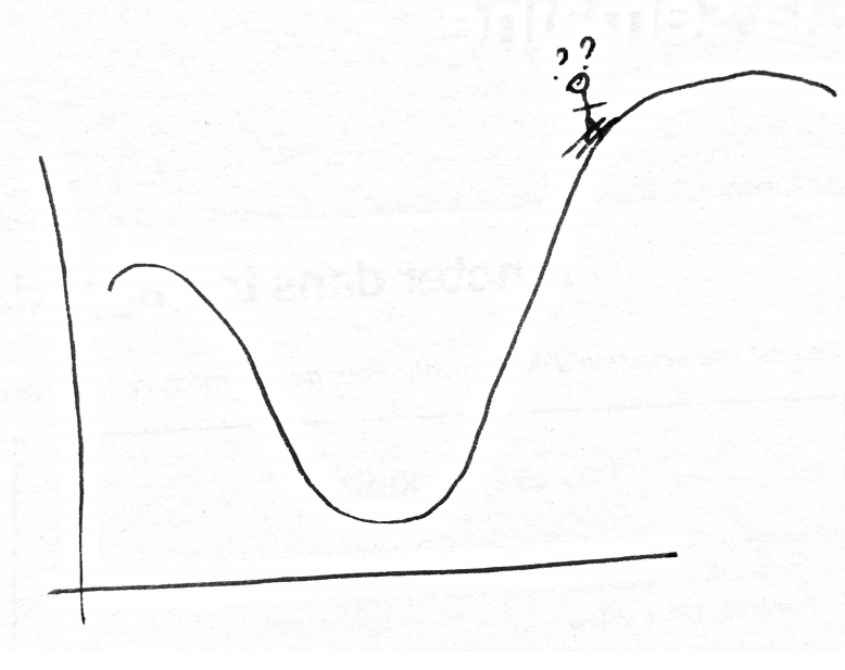
Your approach will be to face the descending slope, and boom you go ahead in this direction for a few minutes.
..
A few minutes later, you’re in a new place.
Once again, you face the descending slope and go ahead for another couple of minutes.
And again.. and again.
After some time, since you keep going down, you will be at the lowest point. Inevitably.
Easy!
What about the math?
Mathematically, the slope is the derivative:
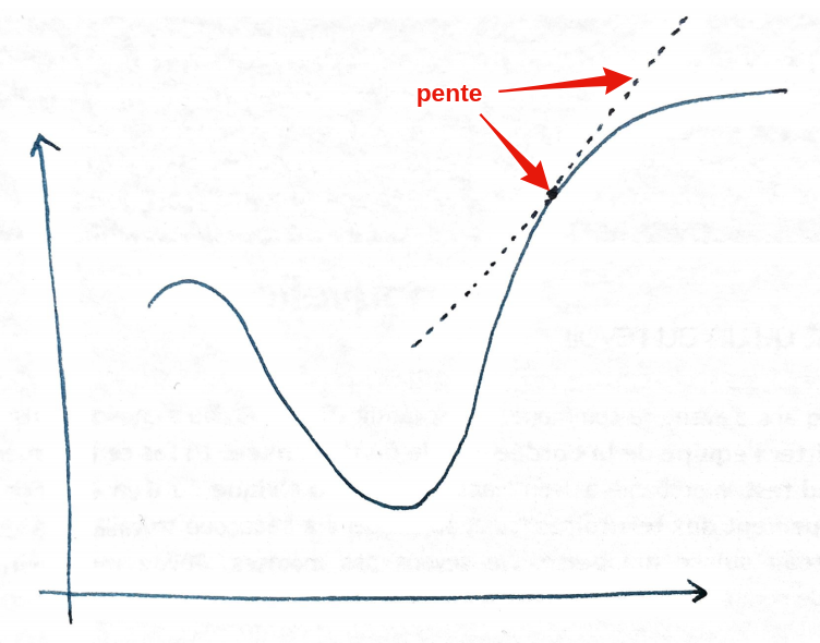
The value of the derivative is the inclination of the slope at a specific point.
So:
- If the derivative is positive, it means the slope goes up (when going to the right!)
- If the derivative is negative, it means the slope goes down.
- If the derivative is equal to \(0\), it means it doesn’t go up or down.
Once you have the value of the slope, what do you do?
You go in the opposite direction!
- Positive derivative => Go to the left.
- Negative derivative => Go to the right.
If you got it, you know that on the drawing, we must go… to the left!
By how much?
But… should we do one step, two steps, or more? For how long?
In fact, we would like to do just one step, then reassess the situation, change direction, do another step, etc.
But this leads to a LOT of decisions, meaning it’s computationally heavy. Hence the algorithm will be too slow.
On the other hand, if you do too many steps at once, you’re at risk of going too far. Then you must go back, maybe going too far again, and so on, and never find the minimum.
So, you have to find a middle ground.
You do that by specifying what we call the learning rate. We’ll come back to this guy again later.
But… the maths?
Let’s take a concrete example, and let’s stop the ugly drawings.
Consider the following function:
\[f(x) = 2x^2 \cos(x) - 5x\]import numpy as np
def f(x):
return 2 * x * x * np.cos(x) - 5 * xAnd let’s study it on the [-5, 5] interval:
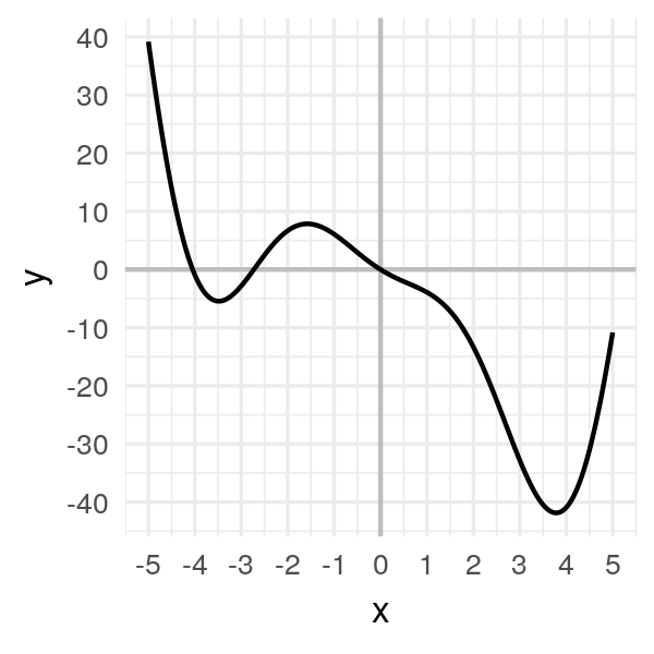
Our goal is to find the minimum, the one you see on the right, with \(x\) between 3 and 4.
We could, in this simple case, compute the derivative, solve \(f'(x) = 0\), etc. But our goal is to understand gradient descent, so let’s do it!
There are 3 steps:
- Take a random point \(x_0\).
- Compute the value of the slope \(f'(x_0)\).
- Walk in the direction opposite to the slope: \(x_1 = x_0 - \alpha * f'(x_0)\). Here, \(\alpha\) is this learning rate we mentioned earlier. And the minus sign enables us to go in the opposite direction.
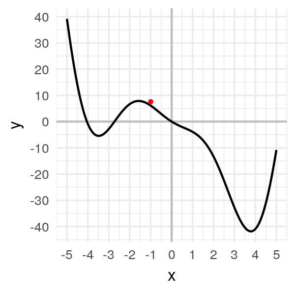
Step 1: Take a random point \(x_0 = -1\). It gives us \(f(x_0) = 6.08\).
x = [-1.]
f(x[0])
# 6.08060
I will draw a big red ball at these coordinates:
Step 2: Compute the slope.
def df(x):
    return 4 * x * np.cos(x) - 2 * x * x * np.sin(x) - 5

slope = df(x[0])
slope
# -5.47827
We have a negative slope of \(-5.23913\).
Step 3: We walk in the opposite direction: \(x_1 = x_0 - \alpha * f'(x_0)\).
What’s \(\alpha\) by the way and how to choose it?
Let’s take \(\alpha = 0.05\) for now. We’ll test other values later on.
alpha = 0.05

x.append(x[0] - alpha * slope)
x[1]
# -0.72609
We get a new value for our new point! Let’s display it:

We moved.. a little bit.
This is an iterative approach, so it’s okay.
Let’s repeat it several times to get the minimum:
x.append(x[1] - alpha * df(x[1]))
x[2]
# -0.40250
We’re moving.. slowly!
After a dozen iterations, we obtain convergence:
x = [-1.]
for i in range(20):
    x.append(x[i] - alpha * df(x[i]))
x
# [-1.0, -0.7260866373071617, -0.4024997370140509, -0.08477906213634434,
# 0.18205499002642517, 0.39684580640116923, 0.5797318757542436,
# 0.7511409760238664, 0.929843593497496, 1.1379425635322518,
# 1.4100262396071885, 1.8111367982460322, 2.4659523010837896,
# 3.481091120446543, 3.9840239754024296, 3.5799142362878964,
# 3.9342838641256046, 3.6341484369757358, 3.900044342976242,
# 3.670089111844099, 3.8747793435314155]
Our little ball finally gets to the minimum and stay there, at \(x = 3.8\).
Most common pitfalls
Ok.
Now, we know how gradient descent works.
On a simple example.
But the reality is often more complicated.
Especially:
- How to find a good value for the learning rate?
- How to solve the vanishing gradient problem?
- What to do in case of local minima?
Let’s answer these questions!
How to find a good value for the learning rate?
In the previous example, we took \(\alpha = 0.05\).
Why?
..
Ok, I’ll admit it. I cheated.
I had tested this value and I knew it worked well.
In fact, it’s hard to find a good value because:
- If \(\alpha\) is too big, you’ll move more quickly, but you have a high risk that the algorithm will never converge.
- If \(\alpha\) is too small, you’ll move slowly.. so slowly you might just lose patience and never reach the minimum.
The latter is to be taken seriously.
When you’re doing Deep Learning and it takes 20 days to train your model just because the learning rate is too small.. yea, you can’t always wait forever.
See what happens if we take \(\alpha = 0.001\):

Ugh..
I had to speed up the animation, otherwise you’d be bored to death.
Instead of getting to the minimum in 15 iterations, you get there in 75 iterations! That’s 5 times longer!
Again, the impact is small with this example. But with deep learning, that makes a huge difference.
Now, see if you take \(\alpha = 0.2\):
Now, the problem is the opposite.
The algorithm has become unstable and move so fast that it always goes so far.
Eventually… it’ll never get to the minimum.
:(
Unfortunately, there is no magic bullet to find the perfect learning rate.
To find a good value, you have to test several values and pick the best.
How to solve the vanishing gradient problem?
There are too frequent problems in Deep Learning: exploding gradient and vanishing gradient.
In the first case, it’s similar to having a too big learning rate. The algorithm is unstable and never converges.
With Deep Learning, it can happen when you’re network is too deep. Since the gradients from each layer get multiplied with each other, you quickly obtain a gradient that explodes exponentially.
For the vanishing gradient, it’s the opposite.
The gradient becomes so small that the skier barely moves anymore.
It can happen if the learning rate is too small, as we discussed earlier.
But it can also happen if the skier is stuck on a flat line.
Take this function:
\[f(x) = \arctan(x^2)\]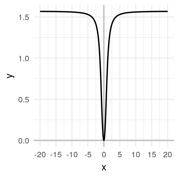
It’s clear that the minimum is at \(x = 0\).
But suppose the initial random point we pick is very far from \(0\), like \(-20\).
Even if I pick a big learning rate (compared to previous examples), like \(\alpha = 1\), the algorithm is very long to converge:
In this example, we can still find the minimum. But with a more complex function that has flat lines in some places AND is very curvy in other places… it becomes a mess.
In this case, whatever value you take for the learning rate, you’ll be in trouble.
Either a very slow convergence or an unstable algorithm.
In Deep Learning, we partially solved this issue by using ReLU functions.
What to do in case of local minima?
Consider another function:
\[f(x) = x \cos(x)\]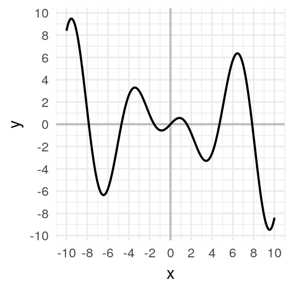
The issue with this one is that there are a lot of local minima, i.e. minima that are not the global minimum.
Look at a few examples where the initial point varies:

Notice the final convergence point depends a lot on the initial point.
Sometimes it’ll find the global minimum. Other times.. not.
To avoid this problem, the best way is to run the algorithms multiple times and keep the best minimum of all times. But, of course, it takes a long time to run.
What next?
In this article, you learn:
- What gradient descent is
- How it works mathematically
- And how to prevent the most common pitfalls
If you want to dive deeper, I invite you to try by yourself with some machine learning algorithms.
For example, start with logistic regression!
That’s what I’ll do in a future article…
Comments
Ben
Thanks for this explanation. I am amazed about the parts alpha and the derivative that work so well together in the formula, that you can choose a reasonable alpha and the iterations of gradient descent will get smaller and smaller increasing your chances of hitting the minimum. However, I’m somewhat skeptical that one could find and alpha and derivative so that the difference taken from the theta would ever hit zero on the nose. I can see algorithms getting close often, but to be perfectly zero seems like your basic trial and error task. That is of course the minimum is a nice round number.
Charles
You have a good point!
Will we hit the absolute minimum exactly? No, until we do many iterations.
Do we need it? Not really, as long as we’re close enough.
For simple problems such as the one I describe in the article, that’s a problem that can be solved exactly.
But for huge problems in high dimensions, such as the ones you get when learning a neural networks, gradient descent is THE way to go.
vihari
can you share your article of logistic regression.i am unable to find it..thanks
Charles
Hi Vihari! Unfortunately.. I haven’t written it yet. (I know :( I don’t publish enough!)
Leave a Comment
Required fields are marked *